Difference between revisions of "NumLib Documentation"
| Line 2,014: | Line 2,014: | ||
end. | end. | ||
</syntaxhighlight> | </syntaxhighlight> | ||
| + | |||
=== Beta function === | === Beta function === | ||
| Line 2,028: | Line 2,029: | ||
* The calculation is based on the logarithms of the gamma function and therefore does not suffer from the overflow issues of the gamma function. | * The calculation is based on the logarithms of the gamma function and therefore does not suffer from the overflow issues of the gamma function. | ||
| − | {{Note|The function <code>beta</code> is not available in fpc v3.0.x | + | {{Note|The function <code>beta</code> is not available in fpc v3.0.x or older.}} |
| − | |||
=== Incomplete beta function === | === Incomplete beta function === | ||
Revision as of 17:21, 25 April 2017
UNDER CONSTRUCTION
Introduction
NumLib is a colletion of routines for numerical mathematics. It was written by C.J.J.M. van Ginneken, W.J.P.M. Kortsmit, and L. Reij at the Technical University of Einhoven (Netherlands) and donated to the Free Pascal project. Its beginnings date back to 1965. Originally written in Algol 60, ported to poorly formatted Pascal with strange procedure names, it is hard stuff, in particular because an official documentation is not readily available (well... -- Dutch documentation files in TeX can be found at http://www.stack.nl/~marcov/numlib/).
But after all, this library contains a series of very useful routines:
- Calculation of special functions
- Solution of systems of linear equations
- Finding roots of equations
- Fitting routines
- Matrix inversion
- Calculation of Eigen values
Therefore, it is the intention of this wiki article to create some useful documentation. Each routine described here was tested and its description will be accompanied by a working code example.
Data types and declarations (unit typ)
Basic floating point type, ArbFloat
In NumLib, a new type ArbFloat is defined which is used as floating point type throughout the entire library. This allows to switch between IEEE Double (64bit) and Extended(80bit) (though big endian state is unknown at present).
At the time of this writing the Define ArbExtended is enabled, and therefore ArbFloat is the type extended.
In order to change the floating point type define or undefine ArbExtended and add the machineconstants change to the type selected.
Basic integer type, ArbInt
Because in plain FPC mode the type Integer is 16-bits (for TP compatibility), and in Delphi 32-bits, all integers were changed to ArbInt. The basic idea is the same as with ArbFloat.
Vectors
NumLib often passes vectors to procedures as one ArbFloat plus some integer value. This ArbFloat value is the first value of an array containing the vector, the integer is the count of elements used from this array. Internally an array type is mapped over the first value in order to access the other array elements. This way both 0- and 1-based arrays as well as static and dynamic arrays can be passed to the functions and procedures of NumLib.
procedure DoSomething(var AVector: ArbFloat; n: Integer);
type
  TLocalVector = array[0..MaxElements] of ArbFloat;
var
  i: Integer;
  x: TLocalVector absolute AVector;
begin
  for i:=0 to n-1 do
    // do something with x[i]
end;

var
  x: array[1..100];   // Note: This array begins with index 1!
...
  DoSomething(x[1], 100);
Matrices
A matrix is a two-dimensional arrangement of numbers in m rows and n columns.
- [math]\displaystyle{ {A} = \left[ \begin{array}{cccc} a_{11} & a_{12} & a_{13} & \ldots & a_{1n}\\ a_{21} & a_{22} & a_{23} & \ldots & a_{2n}\\ \vdots & \vdots & \vdots & \ddots & \vdots\\ a_{m1} & a_{m2} & a_{m3} & \ldots & a_{mn} \end{array} \right] }[/math]
The matrix elements aij are addressed by row and column indexes, i and j, respectively. In mathematics, the index values usually start with 1 (i = 1..m, j = 1..n) while in computing the first index is preferred to be 0 (i = 0...m-1, j = 0...n-1).
Generic matrices
In this type of matrix, no assumption is made on symmetry and shape of the data arrangement.
A constant (real) matrix can be declared in Pascal as a two-dimensional array of floating point numbers: A: array[1..m, 1..n] of ArbFloat (or A: array[0..m-1, 0..n-1] of ArbFloat in 0-based index notation). Similarly, a constant complex matrix can be declared as an array[1..m, 1..n] of complex.
When a NumLib procedure needs a matrix the first (top left) matrix element must be passed as a var parameter, along with the number of rows and columns. It is even possible to allocate larger arrays as needed, and in this case the allocated row length (or number of columns) must be specified.
Alternatively a matrix also can be specified as a one-dimensional array. This works because all data are found within the same memory block. The array index, k must be converted to the 2D matrix indexes, i, j:
 k := i * n + j      <==> i = k div n,           j := k mod n          {for 0-based array and matrix indexes}
 k := (i-1) * n + j  <==> i := (k-1) div n + 1,  j := (k-1) mod n + 1  {for 1-based array and matrix indexes}
Using a one-dimensional array is also the correct way to dynamically allocate memory for a matrix. The first idea of using an array of array of ArbFloat will not work because this does not allocate a single memory block. Instead, individual memory blocks will be allocated for the inner array (rows), and these pointers will be stored in the outer array - this way of storing 2D data is not compatible with the requirements of NumLib.
Here is a simple example how to create, populate and read a matrix dynamically
- [math]\displaystyle{ A = \left[ \begin{array}{ccc} 1 & 2 & 3 \\ 4 & 5 & 6 \end{array} \right] }[/math]
var
  A: array of Arbfloat;  // Note: the index in a dynamic array is 0-based.
  ij: Integer;
  i, j: Integer;
  p: ^ArbFloat;
  m, n: Integer;
begin
  m := 2;
  n := 3;
  SetLength(A, m, n);
  A[0] := 1;  A[1] := 2;  A[2] := 3;
  A[3] := 4;  A[4] := 5;  A[5] := 6;

  for i := 0 to m-1 do begin
    for j := 0 to n-1 do begin
      ij := i * n + j;
      Write(A[ij]);
    end;
    WriteLn;
  end;

  // or
  p := @A[0];   // pointer to first array element
  for i:=0 to m - 1 do begin
    for j := 0 to n - 1 do begin
      WriteLn(p^);
      inc(p);   // advance pointer to next array element
    end;
    WriteLn;
  end;
Tridiagonal matrices
A tridiagonal matrix has zero elements everywhere except for the main diagonal and the diagonal immediately above and below it. This way the matrix can be stored more efficiently than a generic matrix because all the empty elements can be dropped. The elements of an n x n square tridiagonal matrix can be stored as three vectors
- an array
lwithn-1elements for the subdiagonal - an array
dwithnelements for the main diagonal, and - an array
uwithn-1elements for the superdiagonal
- [math]\displaystyle{ A= \begin{bmatrix} d[0] & u[0] & & \dots & 0 \\ l[1] & d[1] & u[1] & & \\ & l[2] & d[2] & u[2] & \\ \vdots & & \ddots & \ddots & \ddots \\ & & l[n-1] & d[n-1] & u[n-1] \\ 0 & & & l[n] & d[n] \end{bmatrix} }[/math]
Symmetric tridiagonal matrices
In these tridiagonal matrices, the subdiagonal and superdiagonal elements are equal. Consequently, NumLib requests only two, instead of three, one-dimensional arrays:
- an array
dwithnelements for the main diagonal, and - an array
cwithn-1elements for the superdiagonal and subdiagonal
- [math]\displaystyle{ A= \begin{bmatrix} d[0] & c[1] & & \dots & 0 \\ c[1] & d[1] & c[2] & & \\ & c[2] & d[2] & c[3] & \\ \vdots & & \ddots & \ddots & \ddots \\ & & c[n-1] & d[n-1] & c[n] \\ 0 & & & c[n] & d[n] \end{bmatrix} }[/math]
Complex numbers
NumLib defines the type complex as a Turbo Pascal object. Real and imaginary parts are denoted as xreal and imag, respectively. Methods for basic operations are provided:
type
  complex  = object
    xreal, imag : ArbFloat;
    procedure Init(r, i: ArbFloat);    // Initializes the number with real and imaginary parts r and i, resp
    procedure Add(c: complex);         // Adds another complex number
    procedure Sub(c: complex);         // Subtracts a complex number
    function  Inp(z:complex):ArbFloat; // Calculates the inner product (a.Re * b.Re + a.Im * b.Im)
    procedure Conjugate;               // Conjugates the value (i.e. negates the imaginary part)
    procedure Scale(s: ArbFloat);      // Multiplies real and imaginary part by the real value s
    function  Norm: ArbFloat;          // Calculates the "norm", i.e. sqr(Re) + sqr(Im)
    function  Size: ArbFloat;          // Size = sqrt(Norm)
    function  Re: ArbFloat;            // Returns the real part of the complex number
    procedure Unary;                   // Negates real and imaginary parts
    function  Im: ArbFloat;            // Returns the imaginary part of the complex number
    function  Arg: ArbFloat;           // Calculates the phase phi of the complex number z = x + y i = r exp(i phi)
    procedure MinC(c: complex);        // Converts itself to the minimum of real and imaginary parts of itself and another value, c
    procedure MaxC(c: complex);        // Converts itself to the maximum of real and imaginary ports of itself and another value, c
    procedure TransF(var t: complex);
  end;
The real and imaginary parts of a complex number can also be retrieved by these stand-alone functions:
  function Re(c: complex): ArbFloat;
  function Im(c: complex): ArbFloat;
Basic operations with matrices and vectors (unit omv)
Inner product of two vectors
The result of the inner product of two vectors a = [a1, a2, ... an] and b = [b1, b2, ... bn] (also called "dot product" or "scalar product") is a scalar, i.e. a single number. It is calculated as the sum of the element-by-element products of the vectors. Both vectors must have the same lengths.
- [math]\displaystyle{ \mathbf{a} \cdot \mathbf{b} = \sum_{i=1}^n a_i b_i = a_1 b_1 + a_2 b_2 + \dots + a_n b_n }[/math]
NumLib provides the function omvinp for calculation of the inner product:
function omvinp(var a, b: ArbFloat; n: ArbInt): ArbFloat;aandbare the first elements of 1-dimensional arrays representing the vectors a and b, respectively.ndefines the dimension of the vectors (count of array elements). Both vectors must have the same number of elements.
Example
Calculate the dot product of the vectors a = [0, 1, 2, 2, -1] and b = [3, -1, -2, 2, -1].
program dot_product;

uses
  typ, omv;

const
  n = 5;
  a: array[0..n-1] of ArbFloat = (0, 1, 2, 2, -1);
  b: array[0..n-1] of Arbfloat = (3, -1, -2, 2, -1);

var
  ab: ArbFloat;
  i: Integer;

begin
  ab := omvinp(a[0], b[0], n);

  Write('Vector a = [');
  for i:= Low(a) to High(a) do
    Write(a[i]:5:0);
  WriteLn('  ]');

  Write('Vector b = [');
  for i:= Low(b) to High(b) do
    Write(b[i]:5:0);
  WriteLn('  ]');

  Write('Dot product a b = ');
  WriteLn(ab:0:0);
end.
Product of two matrices
The product of a m x n matrix A and a n x p matrix B is a m x p matrix C in which the elements are calculated as the inner product of the row vectors of A and the column vectors of B (see here for more details):
- [math]\displaystyle{ C_{ij} = \sum_{k=0}^n A_{ik} B_{kj} }[/math]
The NumLib function to perform this multipication is omvmmm ("mmm" = multiply matrix by matrix):
procedure omvmmm(var a: ArbFloat; m, n, rwa: ArbInt;
                 var b: ArbFloat; p, rwb: ArbInt;
var c: ArbFloat; rwc: ArbInt);ais the first element of the first input matrix A. The array will not be changed.mspecifies the number of rows (or: column length) of matrix A.nspecifies the number or columns (or: row length) of matrix A.rwais the allocated row length of matrix A. This means that the array can be allocated larger than actually needed. Of course,rwacannot be smaller thann.
bis the first element of the second input matrix B. Again, this array will not be changed.pspecifies the number or columns (or: row length) of matrix B. The number of rows is already defined by the number of columns of matrix A,n.rwbis the allocated row length of matrix B.rwbcannot be smaller thanp.
cis the first element of the output matrix C. After the calculation, this and the following array elements will contain the elements of the product matrix.- The size of the output matrix is
mrows xpcolumns as set up by the input matrices A and B. rwcis the allocated row length of matrix C.rwccannot be smaller thanp.
- The size of the output matrix is
Example
Calculate the product of the matrices
- [math]\displaystyle{ A = \begin{bmatrix} 3 & \ 5 & 4 & 1 & -4 \\ -2 & \ 3 & 4 & 1 & 0 \\ 0 & \ 1 & -1 & -2 & 5 \end{bmatrix} \ \ \ \ \ B = \begin{bmatrix} 3 & 4 & -2 & 0 \\ 0 & -2 & 2 & 1 \\ -1 & 0 & 3 & 4 \\ -2 & -3 & 0 & 1 \\ 1 & 3 & 0 & -1 \end{bmatrix} }[/math]
program matrix_multiplication;

uses
  typ, omv;

const
  m = 3;
  n = 5;
  p = 4;

  A: array[1..m, 1..n] of ArbFloat = (
    ( 3,  5,  4,  1, -4),
    (-2,  3,  4,  1,  0),
    ( 0,  1, -1, -2,  5)
  );
  B: array[1..n, 1..p] of ArbFloat = (
    ( 3,  4, -2,  0),
    ( 0, -2,  2,  1),
    (-1,  0,  3,  4),
    (-2, -3,  0,  1),
    ( 1,  3,  0, -1)
  );

var
  C: array[1..m, 1..p] of ArbFloat;
  i, j: Integer;

begin
  // Calculate product
  omvmmm(
    A[1,1], m, n, n,
    B[1,1], p, p,
    C[1,1], p
  );

  // Print A
  WriteLn('A = ');
  for i:= 1 to m do begin
    for j := 1 to n do
      Write(A[i, j]:10:0);
    WriteLn;
  end;
  WriteLn;

  // Print B
  WriteLn('B = ');
  for i:= 1 to n do begin
    for j := 1 to p do
      Write(B[i, j]:10:0);
    WriteLn;
  end;
  WriteLn;

  // Print C
  WriteLn('C = A B = ');
  for i:= 1 to m do begin
    for j := 1 to p do
      Write(C[i, j]:10:0);
    WriteLn;
  end;
end.
Product of a matrix with a vector
A matrix A of size m x n multiplied with a vector b of length n yields another vector of length m. The elements of the result vector c are the dot products of the matrix rows with b. Note that the length of vector b must be equal to the number of columns of matrix A.
- [math]\displaystyle{ \begin{align*} \mathbf{c} = A\ \mathbf{b}= \left[ \begin{array}{cccc} a_{11} & a_{12} & a_{13} & \ldots & a_{1n}\\ a_{21} & a_{22} & a_{23} & \ldots & a_{2n}\\ \vdots & \vdots & \vdots & \ddots & \vdots\\ a_{m1} & a_{m2} & a_{m3} & \ldots & a_{mn} \end{array} \right] \ \ \left[ \begin{array}{c} b_1\\ b_2\\ b_3\\ \vdots\\ b_n \end{array} \right] = \left[ \begin{array}{c} a_{11}b_1+a_{12}b_2 + a_{13}b_3 + \cdots + a_{1n} b_n\\ a_{21}b_1+a_{22}b_2 + a_{23}b_3 + \cdots + a_{2n} b_n\\ \vdots\\ a_{m1}b_1+a_{m2}b_2 + a_{m3}b_3 + \cdots + a_{mn} b_n\\ \end{array} \right]. \end{align*} }[/math]
NumLib's procedure for this task is called omvmmv ("mmv" = multiply a matrix with a vector):
procedure omvmmv(var a: ArbFloat; m, n, rwidth: ArbInt; var b, c: ArbFloat);
Example
Calculate the product
- [math]\displaystyle{ \begin{align*} \mathbf{c} = A\ \mathbf{b}= \left[ \begin{array}{cccc} 3 & 5 & 4 & 1 & -4\\ -2 & 3 & 4 & 1 & 0\\ 0 & 1 & -1 & -2 & 5 \end{array} \right] \ \ \left[ \begin{array}{c} 3\\ 0\\ -1\\ -2\\ 1 \end{array} \right] \end{align*} }[/math]
program matrix_vector_multiplication;

uses
  typ, omv;

const
  m = 3;
  n = 5;
  p = 4;

  A: array[1..m, 1..n] of ArbFloat = (
    ( 3,  5,  4,  1, -4),
    (-2,  3,  4,  1,  0),
    ( 0,  1, -1, -2,  5)
  );
  b: array[1..n] of ArbFloat = (
    3, 0, -1, -2, 1
  );

var
  c: array[1..m] of ArbFloat;
  i, j: Integer;

begin
  // Calculate product c = A b
  omvmmv(
    A[1,1], m, n, n,
    b[1],
    c[1]
  );

  // Print A
  WriteLn('A = ');
  for i:= 1 to m do begin
    for j := 1 to n do
      Write(A[i, j]:10:0);
    WriteLn;
  end;
  WriteLn;

  // Print vector b
  WriteLn('b = ');
  for i:= 1 to n do
    Write(b[i]:10:0);
  WriteLn;
  WriteLn;

  // Print result vector c
  WriteLn('c = A b = ');
  for i:= 1 to m do
    Write(c[i]:10:0);
  WriteLn;
end.
Transpose matrix
The transpose matrix AT of matrix A is obtained by flipping rows and columns:
- [math]\displaystyle{ \begin{align*} {A} = \left[ \begin{array}{cccc} a_{11} & a_{12} & a_{13} & \ldots & a_{1n}\\ a_{21} & a_{22} & a_{23} & \ldots & a_{2n}\\ \vdots & \vdots & \vdots & \ddots & \vdots\\ a_{m1} & a_{m2} & a_{m3} & \ldots & a_{mn} \end{array} \right] \ \ \ {A^T} = \left[ \begin{array}{cccc} a_{11} & a_{21} & \ldots & a_{m1}\\ a_{12} & a_{22} & \ldots & a_{m2}\\ a_{13} & a_{23} & \ldots & a_{m3} \\ \vdots & \vdots & \ddots & \vdots \\ a_{1n} & a_{2n} & \ldots & a{mn} \end{array} \right] \end{align*} }[/math]
Use the procedure omvtrm to perform this operation with NumLib:
procedure omvtrm(
  var a: ArbFloat; m, n, rwa: ArbInt;
  var c: ArbFloat; rwc: ArbInt
);adenotes the first element of the input matrix A. The elements of this array are not changed by the procedure.mis the number of rows of matrix A.nis the number of columns of matrix A.rwais the number of allocated columns of A. This way the array of A can be larger than acutally needed.
cis the first element of the transposed matrix AT. It hasnrows andmcolumns.rwcis the number of allocated columns for the transposed matrix.
Example
Obtain the transpose of the 2x4 matrix
- [math]\displaystyle{ {A} = \left[ \begin{array}{cccc} 1 & 2 & 3 & 4 \\ 11 & 22 & 33 & 44 \end{array} \right] }[/math]
program transpose;

uses
  typ, omv;

const
  m = 2;
  n = 4;

  A: array[1..m, 1..n] of ArbFloat = (
    ( 1,  2,  3,  4),
    (11, 22, 33, 44)
  );

var
  C: array[1..n, 1..m] of ArbFloat;
  i, j: Integer;

begin
  // Transpose A
  omvtrm(
    A[1,1], m, n, n,
    C[1,1], m
  );

  // Print A
  WriteLn('A = ');
  for i:= 1 to m do begin
    for j := 1 to n do
      Write(A[i, j]:10:0);
    WriteLn;
  end;
  WriteLn;

  // Print C
  WriteLn('AT = ');
  for i:= 1 to n do begin
    for j := 1 to m do
      Write(C[i, j]:10:0);
    WriteLn;
  end;
end.
Norm of vectors and matrices
A norm is a function which assigns a positive "length" to a vector a or a matrix M.
In case of vectors, NumLib supports these norms:
- The 1-norm of a vector is defined as the sum of the absolute values of the vector components. It is also called "Taxicab" or "Manhattan" norm because it corresponds to the distance that a taxis has to drive in a rectangular grid of streets.
- [math]\displaystyle{ \|a\|_1 = \sum_{i=1}^n |{a_i}| }[/math]
- The 2-norm (also: Euclidian norm) corresponds to the distance of point a from the origin.
- [math]\displaystyle{ \|a\|_2 = \sqrt{\sum_{i=1}^n {a_i}^2} }[/math]
- The maximum infinite norm of a vector is the maximum absolute value of its components.
- [math]\displaystyle{ \|a\|_\infty = \max({a_1}, {a_2}, ... {a_n}) }[/math]
The norms of matrices, as implemented by NumLib, are usually defined by row or column vectors:
- The 1-norm of a matrix is the maximum of the absolute column sums:
- [math]\displaystyle{ \|M\|_1 = \max_{1 \le j \le {n}} \sum_{i=1}^m|M_{ij}| }[/math]
- The maximum infinite norm of a matrix is the maximum of the absolute row sum.
- [math]\displaystyle{ \|M\|_\infty = \max_{1 \le i \le\ m} \sum_{j=1}^n |M_{ij}| }[/math]
- Only the Frobenius norm is calculated by individual matrix elements. It corresponds to the 2-norm of vectors, only the sum runs over all matrix elements:
- [math]\displaystyle{ \|M\|_F = \sqrt{\sum_{i=1}^m \sum_{j=1}^n {M_{ij}}^2} }[/math]
These are the NumLib procedure for calculation of norms:
function omvn1v(var a: ArbFloat; n: ArbInt): ArbFloat;               // 1-norm of a vector
function omvn1m(var a: ArbFloat; m, n, rwidth: ArbInt): ArbFloat;    // 1-norm of a matrix
function omvn2v(var a: ArbFloat; n: ArbInt): ArbFloat;               // 2-norm of a vector
function omvnfm(Var a: ArbFloat; m, n, rwidth: ArbInt): ArbFloat;    // Frobenius norm of a matrix
function omvnmv(var a: ArbFloat; n: ArbInt): ArbFloat;               // Maximum infinite norm of a vector
function omvnmm(var a: ArbFloat; m, n, rwidth: ArbInt): ArbFloat; // Maximum infinite norm of a matrixais the first element of the vector or matrix of which the norm is to be calculatedm, in case of a matrix norm, is the number of matrix rows.nis the number of vector elements in case of a vector norm, or the number of columns in case of a matrix norm.rwidth, in case of a matrix norm, is the allocated count of columns. This way a larger matrix can be allocated than actually needed.
Example
program norm;

uses
  typ, omv;

const
  n = 2;
  m = 4;
  a: array[0..m-1] of ArbFloat = (0, 1, 2, -3);
  b: array[0..m-1, 0..n-1] of Arbfloat = ((3, -1), (-2, 2), (0, -1), (2, 1));

var
  i, j: Integer;

begin
  Write('Vector a = [');
  for i:= Low(a) to High(a) do
    Write(a[i]:5:0);
  WriteLn('  ]');
  WriteLn('        1-norm of vector a: ', omvn1v(a[0], m):0:3);
  WriteLn('        2-norm of vector a: ', omvn2v(a[0], m):0:3);
  WriteLn('  maximum norm of vector a: ', omvnmv(a[0], m):0:3);
  WriteLn;

  WriteLn('Matrix b = ');
  for i:= 0 to m-1 do begin
    for j := 0 to n-1 do
      Write(b[i,j]:5:0);
    WriteLn;
  end;
  WriteLn('        1-norm of matrix b: ', omvn1m(b[0, 0], m, n, n):0:3);
  WriteLn('Forbenius norm of matrix b: ', omvnfm(b[0, 0], m, n, n):0:3);
  WriteLn('  maximum norm of matrix b: ', omvnmm(b[0, 0], m, n, n):0:3);

  ReadLn;
end.
Inverse of a matrix (unit inv)
Generic matrix
Procedure invgen calculates the inverse of an arbitrary (square) nxn matrix with unknown symmetry. The calculation is based on LU decomposition with partial pivoting.
procedure invgen(n, rwidth: ArbInt; var ai: ArbFloat; var term: ArbInt);nindicates the size of the matrix.rwidthis length of the rows of the two-dimensional array which holds the matrix. Normallyn = rwidth, but the matrix could have been declared larger than actually needed; in this caserwidthrefers to the declared size of the 2D array.aiis the first (top-left) element of the matrix in the 2D array. After the calculation the input data are overwritten by the elements of the inverse matrix in case of successful completion (term = 1); in other cases, the matrix elements are undefined.termprovides an error code:- 1 - successful completion, the elements of the inverse matrix can be found at the same place as the input matrix.
- 2 - the inverse could not be calculated because the input matrix is (almost) singular.
- 3 - incorrect input data,
n < 1.
Example
Find the inverse of the matrix
- [math]\displaystyle{ A = \begin{bmatrix} 2 & 5 & 3 & 1 \\ 1 & 4 & 4 & 3 \\ 3 & 2 & 5 & 3 \\ 1 & 4 & 2 & 2 \end{bmatrix} }[/math]
program inv_general_matrix;

uses
  typ, inv, omv;

const
  n = 4;
  D = 5;

var
  // a is the input matrix to be inverted
  a: array[1..n, 1..n] of ArbFloat = (
    (2, 5, 3, 1),
    (1, 4, 4, 3),
    (3, 2, 5, 3),
    (1, 4, 2, 2)
  );
  b: array[1..n, 1..n] of Arbfloat;
  c: array[1..n, 1..n] of ArbFloat;
  term: Integer = 0;
  i, j: Integer;

begin
  // write input matrix
  WriteLn('a = ');
  for i := 1 to n do begin
    for j := 1 to n do
      Write(a[i, j]:10:D);
    WriteLn;
  end;
  WriteLn;

  // Store input matrix because it will be overwritten by the inverse of a
  for i := 1 to n do
    for j := 1 to n do
      b[i, j] := a[i, j];

  // Calculate inverse matrix
  invgen(n, n, a[1, 1], term);

  // write inverse
  WriteLn('a^(-1) = ');
  for i := 1 to n do begin
    for j := 1 to n do
      Write(a[i, j]:10:D);
    WriteLn;
  end;
  WriteLn;

  // Check validity of result by multiplying inverse with saved input matrix
  omvmmm(a[1, 1], n, n, n,     // "mmm" = Multiply Matrix with Matrix
         b[1, 1], n, n,
         c[1, 1], n);

  // write inverse
  WriteLn('a^(-1) x a = ');
  for i := 1 to n do begin
    for j := 1 to n do
      Write(c[i, j]:10:D);
    WriteLn;
  end;
end.
Determinant of a matrix (unit det)
Unit det provides a series of routines for calculation of the determinant of a square matrix. Besides a procedure for general matrices there are also routines optimized for special matrix types (tridiagonal, symmetric).
In order to avoid possible overflows and underflows a factor may be split off during calculation, and the determinant is returned as a floating point number f times a multiplier 8k. In many cases, however, k = 0, and the determinant simply is equal to f.
Determinant of a generic matrix
The determinant of a generic matrix is calculated by the procedure detgen:
procedure detgen(n, rwidth: ArbInt; var a, f: ArbFloat; var k, term: ArbInt);ndetermines the number of rows and columns of the input matrix (it must be square matrix).rwidthspecifies the allocated row length of the input matrix. This takes care of the fact that matrices can be allocated larger than actually needed.ais the first (i.e. top/left) element of the input matrix. The entire matrix must be contained within the same allocated memory block.fandkreturn the determinant of the matrix. The determinant is given by f * 8k. Usually k = 0, and the determinant simply is equal to f.
Example
Calculate the determinant of the 4x4 matrix
- [math]\displaystyle{ A= \left[ \begin{array}{rrrr} 4 & 2 & 4 & 1 \\ 30 & 20 & 45 & 12 \\ 20 & 15 & 36 & 10 \\ 35 & 28 & 70 & 20 \end{array} \right] }[/math]
program determinant_generic_matrix;

uses
  math, typ, det;

const
  n = 4;

const
  a: array[1..n, 1..n] of ArbFloat = (
  ( 4,  2,  4,  1),
  (30, 20, 45, 12),
  (20, 15, 36, 10),
  (35, 28, 70, 20)
  );

var
  f: ArbFloat;
  k: Integer;
  term: Integer = 0;
  i, j: Integer;

begin
  // write input matrix
  WriteLn('A = ');
  for i := 1 to n do begin
    for j := 1 to n do
      Write(a[i, j]:10:0);
    WriteLn;
  end;
  WriteLn;

  // Calculate determinant
  detgen(n, n, a[1, 1], f, k, term);
  if term = 1 then
    WriteLn('Determinant of A = ', f * intpower(8, k):0:9, ' (k = ', k, ')')
  else
    WriteLn('Incorrect input');
end.
Determinant of a tridiagonal matrix
Calculation of the determinant of a tridiagonal matrix is done by the procedure detgtr:
procedure detgtr(n: ArbInt; var l, d, u, f: ArbFloat; var k, term:ArbInt);ndenotes the number of columns and rows of the matrix (it must be square).lspecifies the first element in the subdiagonal of the matrix. This 1D array must be dimensioned to at leastn-1elements.dspecifies the first element along the main diagonal of the matrix. This 1D array must be dimensioned to contain at leastnelements.uspecifies the first element along the superdiagonal of the matrix. The array must be dimensioned to have at leastn-1elements.fandkreturn the determinant of the matrix. The determinant is given by f * 8k. Usually k = 0, and the determinant simply is equal to f.
Example
Calculate the determinant of the matrix
- [math]\displaystyle{ A= \left( \begin{array}{rrrr} 1 & 1 & & \\ 2 & 1 & 1 & \\ & 1 & 1 & 0 \\ & & 1 & 2 \end{array} \right) }[/math]
program determinant_tridiagonal_matrix;

{$mode objfpc}{$H+}

uses
  math, typ, det;

const
  n = 4;

const
  u: array[0..n-2] of ArbFloat = (-1, -1, -1   );       // superdiagonal
  d: array[0..n-1] of ArbFloat = ( 2,  2,  2,  2);      // main diagonal
  l: array[1..n-1] of ArbFloat = (    -1, -1, -1);      // subdiagonal

var
  f: ArbFloat;
  k: Integer;
  term: Integer = 0;
  i, j: Integer;

begin
  // write input matrix
  WriteLn('A = ');
  for i := 0 to n-1 do begin
    for j := 0 to i-2 do
      Write(0.0:5:0);
    if i > 0 then
      Write(l[i]:5:0);
    Write(d[i]:5:0);
    if i < n-1 then
      Write(u[i]:5:0);
    for j:=i+2 to n-1 do
      Write(0.0:5:0);
    WriteLn;
  end;
  WriteLn;

  // Calculate determinant
  detgtr(n, l[1], d[0], u[0], f, k, term);
  if term = 1 then
    WriteLn('Determinant of A = ', f * intpower(8, k):0:9, ' (k = ', k, ')')
  else
    WriteLn('Incorrect input');

  ReadLn;

end.
Solving systems of linear equations (unit sle)
A system of linear equations (or linear system) is a collection of two or more linear equations involving the same set of variables, x1 ... xn.
- [math]\displaystyle{ \begin{cases} a_{11} x_1 + a_{12} x_2 + \dots + a_{1n} x_n = b_1 \\ a_{21} x_1 + a_{22} x_2 + \dots + a_{2n} x_n = b_n \\ \ \ \ \vdots \\ a_{m1} x_1 + a_{m2} x_2 + \dots + a_{mn} x_n = b_m \end{cases} }[/math]
In order to find a solution which satisfies all equations simultaneously the system of equations is usually converted to a matrix equation A x = b, where
- [math]\displaystyle{ A = \left [ \begin{array}{ccc} a_{11} & a_{12} & \dots & a_{1n} \\ a_{21} & a_{22} & \dots & a_{2n} \\ \vdots & \vdots & \ddots & \vdots \\ a_{m1} & a_{m2} & \dots & a_{mn} \end{array} \right ], \ \mathbf{x} = \left [ \begin{array}{c} x_1 \\ x_2 \\ \vdots \\ x_n \end{array} \right ], \ \mathbf{b} = \left [ \begin{array}{c} b_1 \\ b_2 \\ \vdots \\ b_m \end{array} \right ] }[/math]
NumLib offers several procedures to solve the matrix equation depending on the properties of the matrix.
Generic matrix
The most general procedure is slegen. It poses the only requirement that the coefficient matrix A is square.
procedure slegen(n, rwidth: ArbInt; var a, b, x, ca: ArbFloat; var term: ArbInt);nis the number of unknown variables. It must be the same as the number of columns and rows of the coefficent matrix.rwidthidentifies the allocated number of columns of the coefficient matrix. This is useful if the matrix is allocated larger than needed. It is required thatn <= rwidth.ais the first (i.e. top left) element of the coefficient matrix A; the other elements must follow within the same allocated memory block. The matrix will not be changed during the calculation.bis the first element of the array containing the constant vector b. The array length at least must be equal ton. The vector will not be changed during the calculation.xis the first element of the array to receive the solution vector x. It must be allocated to contain at leastnvalues.cais a parameter to describe the accuracy of the solution.termreturns an error code:- 1 - successful completion, the solution vector x is valid
- 2 - the solution could not have been determined because the matrix is (almost) singular.
- 3 - error in input values:
n < 1.
The solution is calculated using Gauss elimination with partial pivoting.
Example
Solve this system of linear equations:
- [math]\displaystyle{ \begin{cases} 4 x_1 + 2 x_2 + 4 x_3 + x_4 = 5 \\ 30 x_1 + 20 x_2 + 45 x_3 + 12 x_4 = 43 \\ 20 x_1 + 15 x_2 + 36 x_3 + 10 x_4 = 31 \\ 35 x_1 + 28 x_2 + 70 x_3 + 20 x_4 = 57 \end{cases} \qquad \Rightarrow \qquad A= \left[ \begin{array}{rrrr} 4 & 2 & 4 & 1 \\ 30 & 20 & 45 & 12 \\ 20 & 15 & 36 & 10 \\ 35 & 28 & 70 & 20 \end{array} \right] , \; \mathbf{b} = \left[ \begin{array}{r} 5 \\ 43 \\ 31 \\ 57 \end{array} \right] }[/math]
program solve_gen;

uses
  typ, sle, omv;

const
  n = 4;
  A: array[1..n, 1..n] of ArbFloat = (
    ( 4,  2,  4,  1),
    (30, 20, 45, 12),
    (20, 15, 36, 10),
    (35, 28, 70, 20)
  );
  b: array[1..n] of ArbFloat = (
    5, 43, 31, 57
  );

var
  x: array[1..n] of ArbFloat;
  b_test: array[1..n] of ArbFloat;
  ca: ArbFloat;
  i, j: Integer;
  term: Integer;

begin
  WriteLn('Solve matrix system A x = b');
  WriteLn;

  // Print A
  WriteLn('Matrix A = ');
  for i:= 1 to n do begin
    for j := 1 to n do
      Write(A[i, j]:10:0);
    WriteLn;
  end;
  WriteLn;

  // Print b
  WriteLn('Vector b = ');
  for i:= 1 to n do
    Write(b[i]:10:0);
  WriteLn;
  WriteLn;

  // Solve
  slegen(n, n, A[1, 1], b[1], x[1], ca, term);

  if term = 1 then begin
    WriteLn('Solution vector x = ');
    for i:= 1 to n do
      Write(x[i]:10:0);
    WriteLn;
    WriteLn;

    // Check solution
    omvmmv(A[1,1], n, n, n, x[1], b_test[1]);

    WriteLn('Check result: A x = (must be equal to b)');
    for i:= 1 to n do
      Write(b_test[i]:10:0);
    WriteLn;
  end
  else
    WriteLn('Error');
end.
Tridiagonal matrix
NumLib offers two specialized procedures for solving a system of linear equations based on a tridiagonal matrix A. Both rely on the memory-optimized storage of tridiagonal matrices as described here. They differ in the internal calculation algorithm and in the behavior with critical matrices.
procedure sledtr(n: ArbInt; var l, d, u, b, x: ArbFloat; var term: ArbInt);
procedure slegtr(n: ArbInt; var l, d, u, b, x, ca: ArbFloat; var term: ArbInt);nis the number of unknown variables. It must be the same as the number of columns and rows of the coefficent matrix.lspecifies the first element in the subdiagonal of the matrix A. This 1D array must be dimensioned to at leastn-1elements.dspecifies the first element along the main diagonal of the matrix A. This 1D array must be dimensioned to contain at leastnelements.uspecifies the first element along the superdiagonal of the matrix A. The array must be dimensioned to have at leastn-1elements.bis the first element of the array containing the constant vector b. The array length at least must be equal ton. The vector will not be changed during the calculation.xis the first element of the array to receive the solution vector x. It must be allocated to contain at leastnvalues.cais a parameter to describe the accuracy of the solution.termreturns an error code:- 1 - successful completion, the solution vector x is valid
- 2 - the solution could not have been determined because the matrix is (almost) singular.
- 3 - error in input values:
n < 1.
sledtr is numerically stable if matrix A fulfills one of these conditions:
- A is regular (i.e. its inverse matrix exists), and A is columnar-diagonally dominant; this means:
- |d1| ≥ |l2|,
- |di| ≥ |ui-1| + |li+1|, i = 2, ..., n-1,
- |dn| ≥ |un-1|
- A is regular, and A is diagonally dominant; this means:
- |d1| ≥ |l2|,
- |di| ≥ |ui| + |li|, i = 2, ..., n-1,
- |dn| ≥ |un|
- A is symmetric and positive-definite.
However, this procedure does not provide the parameter ca from which the accuracy of the determined solution can be evaluated. If this is needed the (less stable) procedure slegtr must be used.
Example
Solve this tridiagonal system of linear equations:
- [math]\displaystyle{ \begin{cases} 188 x_1 - 100 x_2 = 0 \\ -100 x_1 + 188 x_2 -100 x_3 = 0 \\ \vdots \\ -100 x_{n-2} + 188 x_{n-1} - 100 x_n = 0 \\ -100 x_{n-1} + 188 x_n = 0 \end{cases} \qquad \Rightarrow \qquad A= \left[ \begin{array}{rrrrr} 188 & -100 & & & 0 \\ -100 & 188 & -100 & & \\ & \ddots & \ddots & \ddots & \\ & & -100 & 188 & -100 \\ & & & -100 & 188 \\ \end{array} \right] , \; \mathbf{b} = \left[ \begin{array}{r} 88 \\ -12 \\ \vdots \\ -12 \\ 88 \end{array} \right] }[/math]
program solve_tridiag;

uses
  typ, sle;

const
  n = 8;
  u: array[1..n-1] of ArbFloat = (-100, -100, -100, -100, -100, -100, -100      );
  d: array[1..n] of ArbFloat   = ( 188,  188,  188,  188,  188,  188,  188,  188);
  l: array[2..n] of ArbFloat   = (      -100, -100, -100, -100, -100, -100, -100);
  b: array[1..n] of ArbFloat   = (  88,  -12,  -12,  -12,  -12,  -12,  -12,   88);

var
  A: array[1..n, 1..n] of ArbFloat;
  x: array[1..n] of ArbFloat;
  b_test: array[1..n] of ArbFloat;
  ca: ArbFloat;
  i, j: Integer;
  term: Integer;

begin
  WriteLn('Solve tridiagonal matrix system A x = b');
  WriteLn;

  Write('Superdiagonal of A:':25);
  for i := 1 to n-1 do
    Write(u[i]:10:0);
  WriteLn;

  Write('Main diagonal of A:':25);
  for i:= 1 to n do
    Write(d[i]:10:0);
  WriteLn;

  Write('Subdiagonal of A:':25);
  Write('':10);
  for i:=2 to n do
    Write(l[i]:10:0);
  WriteLn;

  Write('Vector b:':25);
  for i:=1 to n do
    Write(b[i]:10:0);
  WriteLn;


  // Solve
  slegtr(n, l[2], d[1], u[1], b[1], x[1], ca, term);
  { or:
  sledtr(n, l[2], d[1], u[1], b[1], x[1], term);
  }

  if term = 1 then begin
    Write('Solution vector x:':25);
    for i:= 1 to n do
      Write(x[i]:10:0);
    WriteLn;

    // Multiply A with x to test the result
    // NumLib does not have a routine to multiply a tridiagonal matrix with a
    // vector... Let's do it manually.
    b_test[1] := d[1]*x[1] + u[1]*x[2];
    for i := 2 to n-1 do
      b_test[i] := l[i]*x[i-1] + d[i]*x[i] + u[i]*x[i+1];
    b_test[n] := l[n]*x[n-1] + d[n]*x[n];

    Write('Check b = A x:':25);
    for i:= 1 to n do
      Write(b_test[i]:10:0);
    WriteLn;
  end
  else
    WriteLn('Error');
end.
Overdetermined systems (least squares)
Unlike the other routines in unit sle which require a square matrix A, slegls can solve linear systems described by a rectangular matrix which has more rows than colums, or speaking in terms of equations, has more equations than unknowns. Such a system generally is not solvable exactly. But an approximate solution can be found such that the sum of squared residuals of each equation, i.e. the norm
[math]\displaystyle{ \|\mathbf{b} - A \mathbf{x}\|_2 }[/math]
is as small as possible. The most prominent application of this technique is fitting of equations to data (regression analysis).
procedure slegls(var a: ArbFloat; m, n, rwidtha: ArbInt; var b, x: ArbFloat; var term: ArbInt);ais the first (i.e. top left) element of an array with the coefficient matrix A; the other elements must follow within the same allocated memory block. The array will not be changed during the calculation.mis the number of rows of the matrix A (or: the number of equations).nis the number of columns of the matrix A (or: the number of unknown variables). n must not be larger than m.rwidthidentifies the allocated number of columns of the coefficient matrix A. This is useful if the matrix is allocated larger than needed. It is required thatn <= rwidth.bis the first element of the array containing the constant vector b. The array length must correspond to the number of matrix rowsm, but the array can be allocated to be larger.xis the first element of the array to receive the solution vector x. The array length must correspond to the number of matrix columnsn, but the array can be allocated to be larger.termreturns an error code:- 1 - successful completion, the solution vector x is valid
- 2 - there is no unambiguous solution because the columns of the matrix are linearly dependant..
- 3 - error in input values:
n < 1, orn>m.
The method is based on reduction of the array A to upper triangle shape through Householder transformations.
Example
Find the least-squares solution for the system A x = b of 4 equations and 3 unknowns with
[math]\displaystyle{ A= \left( \begin{array}{rrr} 1 & 0 & 1 \\ 1 & 1 & 1 \\ 0 & 1 & 0 \\ 1 & 1 & 0 \end{array} \right), \ \ b= \left( \begin{array}{r} 21 \\ 39 \\ 21 \\ 30 \end{array} \right). }[/math]
program solve_leastsquares;

uses
  typ, sle, omv;

const
  m = 4;
  n = 3;

  A: array[1..m, 1..n] of ArbFloat = (
    (1, 0, 1),
    (1, 1, 1),
    (0, 1, 0),
    (1, 1, 0)
  );
  b: array[1..m] of ArbFloat = (
    21, 39, 21, 30);

var
  x: array[1..n] of ArbFloat;
  term: ArbInt;
  i, j: Integer;
  b_test: array[1..m] of ArbFloat;
  sum: ArbFloat;

begin
  WriteLn('Solve A x = b with the least-squares method');
  WriteLn;

  // Display input data
  WriteLn('A = ');
  for i := 1 to m do
  begin
    for j := 1 to n do
      Write(A[i, j]:10:0);
    WriteLn;
  end;
  WriteLn;
  WriteLn('b = ');
  for i := 1 to m do
    Write(b[i]:10:0);
  WriteLn;

  // Calculate and show solution
  slegls(a[1,1], m, n, n, b[1], x[1], term);

  WriteLn;
  WriteLn('Solution x = ');
  for j:= 1 to n do
    Write(x[j]:10:0);
  WriteLn;

  // Calculate and display residuals
  WriteLn;
  WriteLn('Residuals A x - b = ');
  sum := 0;
  omvmmv(a[1,1], m, n, n, x[1], b_test[1]);
  for i:=1 to m do begin
    Write((b_test[i] - b[i]):10:0);
    sum := sum + sqr(b_test[i] - b[i]);
  end;
  WriteLn;

  // Sum of squared residuals
  WriteLn;
  WriteLn('Sum of squared residuals');
  WriteLn(sum:10:0);

  WriteLn;
  WriteLn('----------------------------------------------------------------------------');
  WriteLn;

  // Modify solution to show that the sum of squared residuals increases';
  WriteLn('Modified solution x'' (to show that it has a larger sum of squared residuals)');
  x[1] := x[1] + 1;
  x[2] := x[2] - 1;
  WriteLn;
  for j:=1 to n do
    Write(x[j]:10:0);
  omvmmv(a[1,1], m, n, n, x[1], b_test[1]);
  sum := 0;
  for i:=1 to m do
    sum := sum + sqr(b_test[i] - b[i]);
  WriteLn;
  WriteLn;
  WriteLn('Sum of squared residuals');
  WriteLn(sum:10:0);
end.
Finding the roots of a function (unit roo)
The roots are the x values at which a function f(x) is zero.
Roots of the quadratic equation
The quadratic equation
- [math]\displaystyle{ {z}^2 + {p} {z} + {q} = 0 }[/math]
always has two, not necessarily different, complex roots. These solutions can be determined by the procedure rooqua.
procedure rooqua(p, q: ArbFloat; var z1, z2: complex);pandqare the (real) coefficients of the quadratic equationz1andz2return the two complex roots. See unit typ for the declaration of the typecomplex
Example
Determine the roots of the equation z2 + 2 z + 5 = 0.
program quadratic_equ;

uses
  SysUtils, typ, roo;

var
  z1, z2: complex;

const
  SIGN: array[boolean] of string = ('+', '-');

begin
  rooqua(2, 5, z1, z2);

  WriteLn(Format('1st solution: %g %s %g i', [z1.re, SIGN[z1.im < 0], abs(z1.im)]));
  WriteLn(Format('2nd solution: %g %s %g i', [z2.re, SIGN[z2.im < 0], abs(z2.im)]));
end.
Bisection
In the bisection method two x values a and b are estimated to be around the expected root such that the function values have opposite signs at a and b. The center point of the interval is determined, and the subinterval for which the function has opposite signs at its endpoints is selected for a new iteration. The process ends when a given precision, i.e. interval length, is achieved.
In NumLib, this approach is supported by the procedure roof1r:
procedure roof1r(f: rfunc1r; a, b, ae, re: ArbFloat; var x: ArbFloat; var term: ArbInt);fis the function for which the root is to be determined. It must be a function of one floating point argument (typeArbFloat). The type of the function,rfunc1r, is declared in unittyp.aandbare the endpoints of the test interval. The root must be located between these two values, i. e. the function values f(a) and f(b) must have different signs.aeandredetermine the absolute and relative precision, respectively, with which the root will be determined.reis relative to the maximum of abs(a) and abs(b). Note that precision and speed are conflicting issues. Highest accuracy is achieved ifaeis given asMachEps(see unittyp). Both parameters must not be negative.xreturns the value of the found root.termreturns whether the process has been successful:- 1 - successful termination, a zero point has been found with absolute accuracy
aeor relative accuracyre - 2 - the required accuracy of the root could not be reached; However, the value of x is called the "best achievable" approach
- 3 - error in input parameters:
ae< 0 orre< 0, or f(a)*f(b) > 0
- 1 - successful termination, a zero point has been found with absolute accuracy
Example
The following program determines the square root of 2. This is the x value at which the function f(x) = x^2 - 2 is zero. Since f(1) = 1^2 - 2 = -1 < 0 and f(2) = 2^2 - 2 = 2 > 0 we can assume a and b to be 1 and 2, respectively.
program bisection_demo;

uses
  typ, roo;

function f(x: ArbFloat): ArbFloat;
begin
  Result := x*x - 2;
end;

var
  x: ArbFloat = 0.0;
  term : ArbInt;

begin
  roof1r(@f, 1.0, 2.0, 1e-9, 0, x, term);
  WriteLn('Bisection result ', x);
  WriteLn('sqrt(2)          ', sqrt(2.0));
end.
Numerical integration of a function (unit int)
The NumLib function int1fr calculates the integral of a given function between limits a and b with a specified absolute accuracy ae:
procedure int1fr(f: rfunc1r; a, b, ae: ArbFloat; var integral, err: ArbFloat; var term: ArbInt);fpoints to the function to be integrated. It must be a function of a single real variable (typeArbFloat) and return anArbfloat. See the typerfunc1rdeclared in unit typ.a, bare the limits of integration.aand/orbcan attain the values+/-Infinityfor integrating over an infinite interval. The order ofaandbis handled in the mathematically correct sense.aedetermines the absolute accuracy requested.integrealreturns the value of the integral. It is only valid ifterm = 1.errreturns the achieved accuracy if the specified accuracy could not be reached.termhas the value 2 in this case.termreturns an error code:- 1 - successful termination, the integral could be calculated with absolute accuracy
ae. - 2 - the requested accuracy could not be reached. But the integral is approximated within the accuracy
err. - 3 - incorrect input data:
ae < 0, ora = b = infinity, ora = b = -infinity - 4 - the integral could not be calculated: divergence, or too-slow convergence.
- 1 - successful termination, the integral could be calculated with absolute accuracy
Example
Calculate the integral
- [math]\displaystyle{ \int_a^b \frac 1 {x^2} \mathrm{d}x }[/math]
for several integration limits a and b. Since the function diverges at x = 0 the interval from a to b must not contain this point. The analytic result is [math]\displaystyle{ -1/{b} + 1/{a} }[/math]
program integrate;

uses
  SysUtils, typ, int;

function recipx2(x: ArbFloat): ArbFloat;
begin
  Result := 1.0 / sqr(x);
end;

function integral_recipx2(a, b: ArbFloat): Arbfloat;
begin
  if a = 0 then
    a := Infinity
  else if a = Infinity then
    a := 0.0
  else
    a := -1/a;
  if b = 0 then
    b := Infinity
  else if b = Infinity then
    b := 0.0
  else
    b := -1/b;
  Result := b - a;
end;

procedure Execute(a, b: ArbFloat);
var
  err: ArbFloat = 0.0;
  term: ArbInt = 0;
  integral: ArbFloat = 0.0;
begin
  try
    int1fr(@recipx2, a, b, 1e-9, integral, err, term);
  except
    term := 4;
  end;
  Write('  The integral from ' + FloatToStr(a) + ' to ' + FloatToStr(b));
  case term of
    1: WriteLn(' is ', integral:0:9, ', exected: ', integral_recipx2(a, b):0:9);
    2: WriteLn(' is ', integral:0:9, ', error: ', err:0:9, ', exected: ', integral_recipx2(a, b):0:9);
    3: WriteLn(' cannot be calculated: Error in input data');
    4: WriteLn(' cannot be calculated: Divergent, or calculation converges too slowly.');
  end;
end;

begin
  WriteLn('Integral of f(x) = 1/x^2');
  Execute(1.0, 2.0);
  Execute(1.0, 1.0);
  Execute(2.0, 1.0);
  Execute(1.0, Infinity);
  Execute(-Infinity, -1.0);
  Execute(0.0, Infinity);
  // NOTE: The next line will raise an exception if run in the IDE. This will not happen outside the IDE.
  // Integrate(-1.0, Infinity);
end.
Interpolation and fitting (unit ipf)
Unit ipf contains routines for
- fitting a set of data points with a polynomial,
- interpolating or fitting a set of data points with a natural cubic spline. A spline is a piecewise defined function of polynomials which has a high degree of smoothness at the connection points of the polynomials ("knots"). In case of a natural cubic spline, the polynomials have degree 3 and their second derivative is zero at the first and last knot.
Fitting means: determine an approximating smooth function such that the deviations from the data points are at minimum.
Interpolation means: determine a function that runs exactly through the data points.
Use of polynomials or splines is recommended unless the data are known to belong to a known function in which there are still some unknown parameters, for example, the data are measurements of the function f(x) = a + b e-c x.
In the most common case, the data contain measurement errors and appear to follow the shape of a "simple" function. Therefore, it is recommended to first try to fit with a low-degree polynomial, e.g. not higher than degree 5. If this is not successful or if the shape of the function is more complicated try to fit with a spline.
If the data contain no (or very little) measurement noise, it is almost always wise to interpolate the data with a spline.
Fitting with a polynomial
For this purpose, the routine ipfpol can be applied. It uses given data points (xi, yi), i = 1, ..., m, and n given coefficients b0, ..., bn to calculate a polynomial
[math]\displaystyle{ \operatorname{p}(x) = b_0 + b_1 x + \dots + b_n x^n }[/math]
In the sense of the least squares fitting, the coefficients b0 ... bn are adjusted to minimize the expression
[math]\displaystyle{ \sum_{i=1}^m {(\operatorname{p}(x) - y_i)^2} }[/math]
procedure ipfpol(m, n: ArbInt; var x, y, b: ArbFloat; var term: ArbInt);mdenotes the number of data points. It is required thatm ≥ 1nis the degree of the polynomial to be fitted. It is required thatn > 0.xis the first element of a one-dimensional array containing the x values of the data points. The array must be allocated to contain at leastmvalues.yis the first element of a one-dimensional array containing the y values of the data points. The array must be dimensioned to contain at leastmvalues.bis the first element of a one-dimenisonal array in which the determined polynomial coefficients are returned iftermis 1. The array must have been dimensioned to provide space for at leastn + 1values. The returned coefficients are ordered from lowest to highest degree.termreturns an error code:- 1 - successful completion, the array
bcontains valid coefficients - 3 - input error:
n < 0, orm < 1.
- 1 - successful completion, the array
After the coefficients b0, ..., bn once have been determined the value of p(x) can be calculated for any x using the procedure spepol from the unit spe.
Example
Fit a polynomial of degree 2 to these data points: [math]\displaystyle{ \begin{array}{ccc} \hline i & x_i & y_i \\ \hline 1 & 0.00 & 1.26 \\ 2 & 0.08 & 1.37 \\ 3 & 0.22 & 1.72 \\ 4 & 0.33 & 2.08 \\ 5 & 0.46 & 2.31 \\ 6 & 0.52 & 2.64 \\ 7 & 0.67 & 3.12 \\ 8 & 0.81 & 3.48 \end{array} }[/math]

program polynomial_fit;

uses
  SysUtils, StrUtils, typ, ipf, spe;

const
  m = 8;
  n = 2;
  x: array[1..m] of Arbfloat = (
    0.00, 0.08, 0.22, 0.33, 0.46, 0.52, 0.67, 0.81
  );
  y: array[1..m] of Arbfloat = (
    1.26, 1.37, 1.72, 2.08, 2.31, 2.64, 3.12, 3.48
  );

var
  b: array[0..n] of ArbFloat;
  i: Integer;
  term: ArbInt;
  xint, yint: ArbFloat;
begin
  WriteLn('Fitting a polynomial of degree 2: p(x) = b[0] + b[1] x + b[2] x^2');
  WriteLn;

  WriteLn('Data points');
  WriteLn('i':10, 'xi':10, 'yi':10);
  for i:=1 to m do
    WriteLn(i:10, x[i]:10:2, y[i]:10:2);
  WriteLn;

  // Execute fit
  ipfpol(m, n, x[1], y[1], b[0], term);

  // Display fitted polynomial coefficients
  WriteLn('Fitted coefficients b = ');
  WriteLn(b[0]:10:6, b[1]:10:6, b[2]:10:6);
  WriteLn;

  // Interpolate and display fitted polynomial for some x values
  WriteLn('Some interpolated data');
  WriteLn('':10, 'x':10, 'y':10);
  for i:= 1 to 5 do begin
    xint := 0.2*i;
    yint := spepol(xint, b[0], n);
    WriteLn('':10, xint:10:2, yint:10:2);
  end;
end.
Interpolation with a natural cubic spline
The routine ipfisn can be used for this purpose. It calculates the parameters of the spline. Once these parameters are known, the value of the spline can be calculated at any point using the ipfspn procedure.
Assume that (xi, yi), i = 0, ..., n' are the given data points with x0 < x1 < ... < xn. Then assume a function g(x) which is twice continuously differentiable (i.e., the first and second derivatives exist and are continuous) and which interpolates the data (i.e., g(xi = yi). Imagine g(x) as the shape of a thin flexible bar. Then the bending energy (in first approximation) is proportional to
[math]\displaystyle{ \int_{-\infty}^{\infty} g''(x)^2 dx }[/math]
The interpolating natural spline s can be understood as the function g which minimizes this integral and therefore the bending energy.
The spline s has the following properties:
- s is a cubic polynomial on the interval [xi, xi+1]
- it is twice continuously differentiable on (-∞, ∞)
- s"(x0) = s"(xn) = 0
- on (-∞, x0) and (xn, ∞) s is linear.
procedure ipfisn(n: ArbInt; var x, y, d2s: ArbFloat; var term: ArbInt);- Calculates the second derivatives of the splines at the knots xi.
nis the index of the last data point, i.e. there aren+1data points.xis the first element of the array with the x coordinates of the data points. It must be dimensioned to contain at lastn+1values. The standard declaration would bevar x: array[0..n] of ArbFloat. The data points must be in strictly ascending order, i.e. there must not be any data points for which xi >= xi+1.yis the first element of the array with the y coordinates of the data points. It must be dimensioned to contain at lastn+1values. The standard declaration would bevar y: array[0..n] of ArbFloat.d2sis the first element of the array which receives the second derivatives of the splines at the knots if the returned error codetermis 1. Note that the array does not contain values for the first and last data point because they are automatically set to 0 (natural splines). Therefore the array must be dimensioned to contain at leastn-1elements. The standard declaration would be:var d2s: array[1..n-1] of ArbFloattermreturns an error code:- 1 - successful completion, the array beginning at
d2scontains valid data - 2 - calculation of the second derivatives was not successful
- 3 - incorrect input parameters: n ≤ 1, or xi ≥ xi+1
- 1 - successful completion, the array beginning at
function ipfspn(n: ArbInt; var x, y, d2s: ArbFloat; t: ArbFloat; var term: ArbInt): ArbFloat;- Calculates the value of the spline function at any coordinate t. The calculation uses the second derivatives determined by
ipnisn. n,x,y,d2shave the same meaning as abovetermreturns an error code:- 1 - successful completion
- 3 - The calculation could not be executed because n ≤ 1.
Example
Interpolate a natural cubic spline through the following data points: [math]\displaystyle{ \begin{array}{ccc} \hline i & x_i & y_i \\ \hline 0 & 0.00 & 0.980 \\ 1 & 0.09 & 0.927 \\ 2 & 0.22 & 0.732 \\ 3 & 0.34 & 0.542 \\ 4 & 0.47 & 0.385 \\ 5 & 0.58 & 0.292 \\ 6 & 0.65 & 0.248 \\ 7 & 0.80 & 0.179 \\ 8 & 0.93 & 0.139 \end{array} }[/math]

program spline_interpolation;

uses
  typ, ipf;

const
  n = 8;
  x: array[0..n] of Arbfloat = (
    0.00, 0.09, 0.22, 0.34, 0.47, 0.58, 0.65, 0.80, 0.93
  );
  y: array[0..n] of Arbfloat = (
    0.990, 0.927, 0.734, 0.542, 0.388, 0.292, 0.248, 0.179, 0.139
  );

var
  s: array[0..n] of ArbFloat;
  d2s: array[1..n-1] of ArbFloat;
  i: Integer;
  term: ArbInt;
  xint, yint: ArbFloat;
begin
  WriteLn('Interpolation with a natural cubic spline');
  WriteLn;

  WriteLn('Data points');
  WriteLn('i':10, 'xi':10, 'yi':10);
  for i:=0 to n do
    WriteLn(i:10, x[i]:10:2, y[i]:10:3);
  WriteLn;

  // Interpolation
  ipfisn(n, x[0], y[0], d2s[1], term);

  // Display 2nd derivatives of splines at xi
  WriteLn('s"(xi)');
  Write(0.0:10:6);      // 2nd derivative of 1st point is 0
  for i:=1 to n-1 do
    Write(d2s[i]:10:6);
  WriteLn(0.0:10:6);    // 2nd derivative of last point is 0
  WriteLn;

  // Interpolate for some x values
  WriteLn('Some interpolated data');
  WriteLn('':10, 'x':10, 'y':10);
  for i:= 1 to 5 do begin
    xint := 0.2 * i;
    yint := ipfspn(n, x[0], y[0], d2s[1], xint, term);
    WriteLn('':10, xint:10:2, yint:10:2);
  end;

end.
Fitting with a natural cubic spline
The routine ipffsn can be used for this purpose. This routine calculates the spline-fit parameters. Once these parameters are known the value of the spline can be calculated at any point using the procedure ipfspn.
Following the model with the bending energy in the previous chapter the calculated fit minimizes
[math]\displaystyle{ \int_{-\infty}^{\infty} g''(x)^2 dx + \lambda \sum_{i=0}^n (g(x_i) - y_i)^2 }[/math]
where the parameter λ must be determined. It is a measure of the compromise between the "smoothness" of the fit - which is measured by the integral (the bending energy) - and the deviation of the fit to the given data - which is measured by the sum of squares. The solution is again a natural cubic spline.
Warning: The procedure ipffsn is buggy and crashes. Therefore, it is not documented at the moment.
Special functions (unit spe)
Evaluation of a polynomial
Horner's scheme provides an efficient method for evaluating a polynomial at a specific x value:
- [math]\displaystyle{ \operatorname{p}(x) = a_0 + a_1 x + a_2 x^2 + ... + a_n x^n \ \Rightarrow \ \operatorname{p}(x) = a_0 + x (a_1 + x (a_2 + \dots + x (a_{n-1} + x a_n))) }[/math]
This method is applied in NumLib's procedure spepol:
function spepol(x: ArbFloat; var a: ArbFloat; n: ArbInt): ArbFloat;xis the argument at which the polynomial is evaluated.ais the first element of an array containing the polynomial coefficients a0, a1, a2, ... an. The coefficient must be ordered from lowest to highest degree.nis the degree of the polynomial, i.e. there aren+1elements in the array.
Example
Evaluate the polynomial
- [math]\displaystyle{ \operatorname{p}(x) = 2 x^3 - 6 x^2 + 2 x - 1 }[/math]
at x = 3. Note that the terms are not in the correct order for spepol and rearrange them to
- [math]\displaystyle{ \operatorname{p}(x) = -1 + 2 x - 6 x^2 + 2 x^3 }[/math]
program polynomial;

uses
  typ, spe;

const
  n = 3;
  a: array[0..n] of ArbFloat = (-1, 2, -6, 2);

var
  x, y: ArbFloat;
begin
  x := 3.0;
  y := spepol(x, a[0], n);
  WriteLn(y:0:6);
end.
Error function

The error function erf(x) and its complement, the complementary error function erfc(x), are the lower and upper integrals of the Gaussian function, normalized to unity:
- [math]\displaystyle{ \operatorname{erf}(x) = \frac {2} {\sqrt{\pi}} \int_0^x e^{-{t}^2} dt }[/math]
- [math]\displaystyle{ \operatorname{erfc}(x) = \frac {2} {\sqrt{\pi}} \int_x^\infty e^{-{t}^2} dt = {1} - \operatorname{erf}(x) }[/math]
Both functions can be calculated by the NumLib functions speerf and speefc, respectively
function speerf(x: ArbFloat): ArbFloat;   // --> erf(x)
function speefc(x: ArbFloat): ArbFloat;   // --> erfc(x)
Example
A table of some values of the error function and the complementary error function is calculated in the following demo project:
program erf_Table;

uses
  SysUtils, StrUtils, typ, spe;

const
  Wx = 7;
  Wy = 20;
  D = 6;

var
  i: Integer;
  x: ArbFloat;
  fs: TFormatSettings;
begin
  fs := DefaultFormatSettings;
  fs.DecimalSeparator := '.';
  WriteLn('x':Wx, 'erf(x)':Wy+1, 'erfc(x)':Wy+1);
  WriteLn;
  for i:= 0 to 20 do begin
    x := 0.1*i;
    WriteLn(Format('%*.1f %*.*f %*.*f', [
      Wx, x,
      Wy, D, speerf(x),
      Wy, D, speefc(x)
    ], fs));
  end;
end.
Normal distribution

The (cumulative) normal distribution is the integral of the Gaussian function with zero mean and unit standard deviation, i.e.
[math]\displaystyle{ \operatorname{N}(x) = \frac{1}{\sqrt{2\pi}} \int_{-\infty}^{x} \operatorname{exp}(\frac{t^2}{2}) dt = \frac{1}{2}[1 + \operatorname{erf} (\frac{x}{\sqrt{2}})] }[/math]
Suppose a set of random floating point numbers which are distributed according to this formula. Then N(x) measures the probability that a number from this set is smaller than x.
In NumLib, the normal distribution is calculated by the function normaldist:
function normaldist(x: ArbFloat): ArbFloat;xcan take any value between -∞ and +∞.- The function result is between 0 and 1.
The inverse normal distribution of y returns the x value for which the normal distribution N(x) has the value y.
function invnormaldist(y: ArbFloat): ArbFloat;yis allowed only between 0 and 1.- The function can take any value between -∞ and +∞.
normaldist and invnormaldist are not available in fpc 3.0.x and older.
Example
Calculate the probabilities for x = -10, -8, ..., 12 for a normal distribution with mean μ = 2 and standard deviation σ = 5. In order to reduce this distribution to the standard normal distribution implemented by NumLib, we introduce a transformation xr = (x - μ)/σ.
program normdist;

uses
  typ, spe;

const
  mu = 2.0;
  sigma = 5.0;
  x: array[0..12] of ArbFloat = (-10, -8, -6, -4, -2, 0, 2, 4, 6, 8, 10, 12, 14);

var
  xr, y: ArbFloat;
  i: Integer;
begin
  WriteLn('Normal distribution with mean ', mu:0:1, ' and standard deviation ', sigma:0:1);
  WriteLn;
  WriteLn('x':20, 'y':20);

  for i:= 0 to High(x) do begin
    xr := (x[i] - mu) / sigma;
    y := normaldist(xr);
    WriteLn(x[i]:20:1, y:20:6);
  end;
end.
Gamma function

The gamma function is needed by many probability functions. It is defined by the integral
- [math]\displaystyle{ \Gamma({x}) = \int_0^{\infty}t^{x-1} e^{-t} dt }[/math]
NumLib provides two functions for its calculation:
function spegam(x: ArbFloat): ArbFloat;
function spelga(x: ArbFloat): ArbFloat;
The first one, spegam, calculates the function directly. But since the gamma function grows rapidly for even not-too large arguments this calculation very easily overflows.
The second function, spelga calculates the natural logarithm of the gamma function which is more suitable to combinatorial calculations where multiplying and dividing the large gamma values can be avoided by adding or subtracting their logarithms.
Example
The following demo project prints a table of some values of the gamma function and of its logarithm. Note that spegam(x) overflows above about x = 170 for data type extended.
program Gamma_Table;

uses
  SysUtils, StrUtils, typ, spe;

const
  VALUES: array[0..2] of ArbFloat = (1, 2, 5);
  Wx = 7;
  Wy = 30;
  Wln = 20;

var
  i: Integer;
  x: ArbFloat;
  magnitude: ArbFloat;
begin
  WriteLn('x':Wx, 'Gamma(x)':Wy, 'ln(Gamma(x))':Wln);
  WriteLn;
  magnitude := 1E-3;
  while magnitude <= 1000 do begin
    for i := 0 to High(VALUES) do begin
      x := VALUES[i] * magnitude;
      Write(PadLeft(FloatToStr(x), Wx));
      if x <= 170 then  // Extended overflow above 170
        Write(FormatFloat('0.000', spegam(x)):Wy)
      else
        Write('overflow':Wy);
      WriteLn(spelga(x):Wln:3);
      if abs(x-1000) < 1E-6 then
        break;
    end;
    magnitude := magnitude * 10;
  end;
end.
Incomplete gamma function

The lower and upper incomplete gamma functions are defined by
- [math]\displaystyle{ \operatorname{P}({s},{x}) = \frac{1}{\Gamma({s})} \int_0^{x}t^{s-1} e^{-t} dt }[/math]
- [math]\displaystyle{ \operatorname{Q}({s},{x}) = \frac{1}{\Gamma({s})} \int_{x}^{\infty}t^{s-1} e^{-t} dt = 1 - \operatorname{P}({s}, {x}) }[/math]
function gammap(s, x: ArbFloat): ArbFloat;
function gammaq(s, x: ArbFloat): ArbFloat;- The parameter
smust be positive: s > 0 - The argument
xmust not be negative: x ≥ 0 - The function results are in the interval [0, 1].
gammap and gammaq are not available in fpc v3.0.x and older.
Example
The following project prints out a table of gammap and gammaq values:
program IncompleteGamma_Table;

uses
  SysUtils, StrUtils, typ, spe;

const
  s = 1.25;

  Wx = 7;
  Wy = 20;
  D = 6;

var
  i: Integer;
  x: ArbFloat;
  fs: TFormatSettings;
begin
  fs := DefaultFormatSettings;
  fs.DecimalSeparator := '.';
  WriteLn('x':Wx, 'GammaP('+FloatToStr(s,fs)+', x)':Wy+1, 'GammaQ('+FloatToStr(s,fs)+', x)':Wy+1);
  WriteLn;
  for i := 0 to 20 do begin
    x := 0.5*i;
    WriteLn(Format('%*.1f %*.*f %*.*f', [
      Wx, x,
      Wy, D, gammap(s, x),
      Wy, D, gammaq(s, x)
    ], fs));
  end;
end.
Beta function

The Beta function is another basis of important functions used in statistics. It is defined as
- [math]\displaystyle{ \operatorname{B}(a, b) = \frac{{\Gamma(a)}{\Gamma(b)}}{\Gamma(a+b)} = \int_0^1{t^{x-1} (1-t)^{y-1} dt} }[/math]
The NumLib routine for its calculation is
function beta(a, b: ArbFloat): ArbFloat;- The arguments
aandbmust be positive:a > 0andb > 1. - The calculation is based on the logarithms of the gamma function and therefore does not suffer from the overflow issues of the gamma function.
beta is not available in fpc v3.0.x or older.Incomplete beta function

The (regularized) incomplete beta function is defined by
- [math]\displaystyle{ \operatorname{I}_x(a,b) = \frac {1}{\operatorname{B}(ab)} \int_0^x{t^{x-1} (1-t)^{y-1} dt} }[/math]
function betai(a, b, x: ArbFloat): ArbFloat;- The arguments
aandbmust be positive:a > 0andb > 1. xis only allowed to be in the range 0 ≤ x ≤ 1.- The function result is in the interval [0, 1].
The inverse incomplete beta function determines the argument x for which the passed parameter is equal to Ix(a, b):
function invbetai(a, b, y: ArbFloat): ArbFloat;
- The arguments
a and b must be positive: a > 0 and b > 1.
y is only allowed to be in the range 0 ≤ x ≤ 1.- The function result is in the interval [0, 1].
 Note: The functions
 betai and invbetai are not available in fpc v3.0.x and older.
Example
Calculate the incomplete beta function for some values of x, a, b, and apply the result to the inverse incomplete beta function to demonstrate the validity of the calculations.
program incomplete_beta_func;

uses
  SysUtils, typ, spe;

  procedure TestBetai(a, b, x: ArbFloat);
  var
    xc, y: ArbFloat;
  begin
    y := betai(a, b, x);
    xc := invbetai(a, b, y, macheps);
    WriteLn('  x = ', x:0:6, '  --->  y = ', y:0:9, '  --->  x = ', xc:0:6);
  end;

begin
  WriteLn('Incomplete beta function and its inverse');
  WriteLn;
  WriteLn('        y = betai(1, 3, x)      x = invbetai(1, 3, y)');
  TestBetaI(1, 3, 0.001);
  TestBetaI(1, 3, 0.01);
  TestBetaI(1, 3, 0.1);
  TestBetaI(1, 3, 0.2);
  TestBetaI(1, 3, 0.9);
  TestBetaI(1, 3, 0.99);
  TestBetaI(1, 3, 0.999);
  WriteLn;

  WriteLn('        y = betai(1, 1, x)      x = invbetai(1, 1, y)');
  TestBetaI(1, 1, 0.001);
  TestBetaI(1, 1, 0.01);
  TestBetaI(1, 1, 0.1);
  TestBetaI(1, 1, 0.2);
  TestBetaI(1, 1, 0.9);
  TestBetaI(1, 1, 0.99);
  TestBetaI(1, 1, 0.999);
  WriteLn;

  WriteLn('        y = betai(3, 1, x)      x = invbetai(3, 1, y)');
  TestBetaI(3, 1, 0.001);
  TestBetaI(3, 1, 0.01);
  TestBetaI(3, 1, 0.1);
  TestBetaI(3, 1, 0.2);
  TestBetaI(3, 1, 0.9);
  TestBetaI(3, 1, 0.99);
  TestBetaI(3, 1, 0.999);
  WriteLn;
end.
Bessel functions
The Bessel functions are solutions of the Bessel differential equation:
- [math]\displaystyle{ {x}^2 y'' + x y' + ({x}^2 - \alpha^2) {y} = 0 }[/math]
The Bessel functions of the first kind, or cylindrical harmonics, Jα(x), are the solutions which are not singular at the origin, in contrast to the Bessel functions of the second kind, Yα(x). Yα(x) is only defined for x > 0.
Example
- Calculate the probability that random normal-distributed numbers are within 1, 2, and 3 standard deviations around the mean.
- Calculate the maximum deviation of normal-distributed deviates (in units of standard deviations) from the mean at probabilities 0.90, 0.95, 0.98, 0.99 and 0.999.


The solutions for a purely imaginary argument are called modified Bessel functions of the first kind, Iα(x), and modified Bessel function of the second kind, Kα(x). Kα(x) is only defined for x > 0.
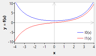
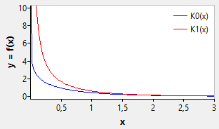
NumLib implements only the solutions for the parameters α = 0 and α = 1:


function spebj0(x: ArbFloat): ArbFloat;     // Bessel function of the first kind, J0 (alpha = 0)
function spebj1(x: ArbFloat): ArbFloat;     // Bessel function of the first kind, J1 (alpha = 1)

function speby0(x: ArbFloat): ArbFloat;     // Bessel function of the second kind, Y0 (alpha = 0)
function speby1(x: ArbFloat): ArbFloat;     // Bessel function of the second kind, Y1 (alpha = 1)

function spebi0(x: ArbFloat): ArbFloat;     // modified Bessel function of the first kind, I0 (alpha = 0)
function spebi1(x: ArbFloat): ArbFloat;     // modified Bessel function of the first kind, I1 (alpha = 1)

function spebk0(x: ArbFloat): ArbFloat;     // modified Bessel function of the second kind, K0 (alpha = 0)
function spebk1(x: ArbFloat): ArbFloat;     // modified Bessel function of the second kind, K1 (alpha = 1)
Other functions
The unit spe contains some other functions which will not be documented here because they are already available in th FPC's standard unit math.
Function

  Equivalent function
 in math

Description


function speent(x: ArbFloat): LongInt;

floor(x)

Entier function, calculates first integer smaller than or equal to x


function spemax(a, b: Arbfloat): ArbFloat;

max(a, b)

Maximum of two floating point values


function spepow(a, b: ArbFloat): ArbFloat;

power(a, b)

Calculates ab


function spesgn(x: ArbFloat): ArbInt;

sign(x)

Returns the sign of x (-1 for x < 0, 0 for x = 0, +1 for x > 0)


function spears(x: ArbFloat): ArbFloat;

arcsin(x)

Inverse function of sin(x)


function spearc(x: ArbFloat): ArbFloat;

arccos(x)

Inverse function of cos(x)


function spesih(x: ArbFloat): ArbFloat;

sinh(x)

Hyperbolic sine


function specoh(x: ArbFloat): ArbFloat;

cosh(x)

Hyperbolic cosine


function spetah(x: ArbFloat): ArbFloat;

tanh(x)

Hyperbolic tangent


function speash(x: ArbFloat): ArbFloat;

arcsinh(x)

Inverse of the hyperbolic sine


function speach(x: ArbFloat): ArbFloat;

arccosh(x)

Inverse of the hyperbolic cosine


function speath(x: ArbFloat): ArbFloat;

arctanh(x)

Inverse of the hyperbolic tangent