NumLib Documentation

UNDER CONSTRUCTION

Introduction

NumLib is a colletion of routines for numerical mathematics. It was written by C.J.J.M. van Ginneken, W.J.P.M. Kortsmit, and L. Reij at the Technical University of Einhoven (Netherlands) and donated to the Free Pascal project. Its beginnings date back to 1965. Originally written in Algol 60, ported to poorly formatted Pascal with strange procedure names, it is hard stuff, in particular because an official documentation is not available.

But after all, this library contains a series of very useful routines:

• Calculation of special functions
• Solution of systems of linear equations
• Finding roots of equations
• Fitting routines
• Matrix inversion
• Calculation of Eigen values

Therefore, it is the intention of this wiki article to create some useful documentation. Each routine described here was tested and its description will be accompanied by a working code example.

Data types and declarations (unit typ)

Basic floating point type, ArbFloat

In NumLib, a new type ArbFloat is defined which is used as floating point type throughout the entire library. This allows to switch between IEEE Double (64bit) and Extended(80bit) (though big endian state is unknown at present).

At the time of this writing the Define ArbExtended is enabled, and therefore ArbFloat is the type extended.

In order to change the floating point type define or undefine ArbExtended and add the machineconstants change to the type selected.

Basic integer type, ArbInt

Because in plain FPC mode the type Integer is 16-bits (for TP compatibility), and in Delphi 32-bits, all integers were changed to ArbInt. The basic idea is the same as with ArbFloat.

Vectors and matrices

NumLib often passes vectors to procedures as one ArbFloat plus some integer value. This ArbFloat value is the first value of an array containing the vector, the integer is the count of elements used from this array. Internally an array type is mapped over the first value in order to access the other array elements. This way both 0- and 1-based arrays as well as static and dynamic arrays can be passed to the functions and procedures of NumLib.

procedure DoSomething(var AVector: ArbFloat; n: Integer);
type
  TLocalVector = array[0..MaxElements] of ArbFloat;
var
  i: Integer;
  x: TLocalVector absolute AVector;
begin
  for i:=0 to n-1 do
    // do something with x[i]
end;

var
  x: array[1..100];   // Note: This array begins with index 1!
...
  DoSomething(x[1], 100);

Similarly, a matrix is passed in the same way as the value of the first ArbFloat value of the first row/column, plus two integers specifying the number of rows and columns. Data are considered to be arranged in rows. Memory must be allocated in a single block to hold all rows, i.e. each row must follow the previous one immediately. Static allocations (array[1..n, 1..n] of ArbFloat) do fulfill this requirement. Dynamically allocated arrays according to array of array of ArbFloat, however, are not suitable because each row is allocated independently of the others, and administrative information may be found at the beginning of the data part of each row. The only way to dynamically allocate memory for a matrix compatible with the requirements of NumLib is to allocate a one-dimensional array and calculate the array index from the column and row index:

// Assume a mxn matrix M[i,j] allocated as a 1-D array A, i=0..m-1, j=0..n-1, 
var
  A: array of ArbFloat;
  ij: Integer;
begin
  SetLength(A, n*m);
  ij := i*n + j;
  Mij := A[ij];  // read M[i, j]
...

Complex numbers

NumLib defines the type complex as a TP object. Real and imaginary parts are denoted as xreal and imag, respectively. Methods for basic operations are provided:

type
  complex  = object
    xreal, imag : ArbFloat;
    procedure Init(r, i: ArbFloat);    // Initializes the number with real and imaginary parts r and i, resp
    procedure Add(c: complex);         // Adds another complex number 
    procedure Sub(c: complex);         // Subtracts a complex number
    function  Inp(z:complex):ArbFloat; // Calculates the inner product (a.Re * b.Re + a.Im * b.Im)
    procedure Conjugate;               // Conjugates the value (i.e. negates the imaginary part)
    procedure Scale(s: ArbFloat);      // Multiplies real and imaginary part by the real value s
    function  Norm: ArbFloat;          // Calculates the "norm", i.e. sqr(Re) + sqr(Im) 
    function  Size: ArbFloat;          // Size = sqrt(Norm) 
    function  Re: ArbFloat;            // Returns the real part of the complex number
    procedure Unary;                   // Negates real and imaginary parts
    function  Im: ArbFloat;            // Returns the imaginary part of the complex number
    function  Arg: ArbFloat;           // Calculates the phase phi of the complex number z = x + y i = r exp(i phi)
    procedure MinC(c: complex);        // Converts itself to the minimum of real and imaginary parts
    procedure MaxC(c: complex);        // Converts itself to the maximum of real and imaginary ports
    procedure TransF(var t: complex);
  end;

The real and imaginary parts of a complex number can also be retrieved by these stand-alone functions:

  function Re(c: complex): ArbFloat;
  function Im(c: complex): ArbFloat;

Basic operations with matrices and vectors (unit omv)

Multiplication of two matrices

The product of a m x n matrix A and a n x p matrix B is a m x p matrix C in which the elements are calculated as the inner product of the row vectors of A and the column vectors of B (see here for more details):

The NumLib function to perform this multipication is omvmmm ("mmm" = multiply matrix by matrix):

procedure omvmmm(var a: ArbFloat; m, n, rwa: ArbInt;
                 var b: ArbFloat; p, rwb: ArbInt;
                 var c: ArbFloat; rwc: ArbInt);

• a is the first element of the first input matrix A. The array will not be changed.
  • m specifies the number of rows (or: column length) of matrix A.
  • n specifies the number or columns (or: row length) of matrix A.
  • rwa is the allocated row length of matrix A. This means that the array can be allocated larger than actually needed. Of course, rwa cannot be smaller than n.

• b is the first element of the second input matrix B. Again, this array will not be changed.
  • p specifies the number or columns (or: row length) of matrix B. The number of rows is already defined by the number of columns of matrix A, n.
  • rwb is the allocated row length of matrix B. rwb cannot be smaller than p.

• c is the first element of the output matrix C. After the calculation, this and the following array elements will contain the elements of the product matrix.
  • The size of the output matrix is m rows x p columns as set up by the input matrices A and B.
  • rwc is the allocated row length of matrix C. rwc cannot be smaller than p.

Example

Calculate the product of the matrices

program matrix_multiplication;

uses
  typ, omv;

const
  m = 3;
  n = 5;
  p = 4;

  A: array[1..m, 1..n] of ArbFloat = (
    ( 3,  5,  4,  1, -4),
    (-2,  3,  4,  1,  0),
    ( 0,  1, -1, -2,  5)
  );
  B: array[1..n, 1..p] of ArbFloat = (
    ( 3,  4, -2,  0),
    ( 0, -2,  2,  1),
    (-1,  0,  3,  4),
    (-2, -3,  0,  1),
    ( 1,  3,  0, -1)
  );

var
  C: array[1..m, 1..p] of ArbFloat;
  i, j: Integer;

begin
  // Calculate product
  omvmmm(
    A[1,1], m, n, n,
    B[1,1], p, p,
    C[1,1], p
  );

  // Print A
  WriteLn('A = ');
  for i:= 1 to m do begin
    for j := 1 to n do
      Write(A[i, j]:10:0);
    WriteLn;
  end;
  WriteLn;

  // Print B
  WriteLn('B = ');
  for i:= 1 to n do begin
    for j := 1 to p do
      Write(B[i, j]:10:0);
    WriteLn;
  end;
  WriteLn;

  // Print C
  WriteLn('C = A B = ');
  for i:= 1 to m do begin
    for j := 1 to p do
      Write(C[i, j]:10:0);
    WriteLn;
  end;
end.

Inverse of a matrix (unit inv)

General matrix

Procedure invgen calculates the inverse of an arbitrary (square) nxn matrix with unknown symmetry. The calculation is based on LU decomposition with partial pivoting.

procedure invgen(n, rwidth: ArbInt; var ai: ArbFloat; var term: ArbInt);

• n indicates the size of the matrix.
• rwidth is length of the rows of the two-dimensional array which holds the matrix. Normally n = rwidth, but the matrix could have been declared larger than actually needed; in this case rwidth refers to the declared size of the 2D array.
• ai is the first (top-left) element of the matrix in the 2D array. After the calculation the input data are overwritten by the elements of the inverse matrix in case of successful completion (term = 1); in other cases, the matrix elements are undefined.
• term provides an error code:
  • 1 - successful completion, the elements of the inverse matrix can be found at the same place as the input matrix.
  • 2 - the inverse could not be calculated because the input matrix is (almost) singular.
  • 3 - incorrect input data, n < 1.

Example

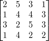
Find the inverse of the matrix

program inv_general_matrix;

uses
  typ, inv, omv;

const
  n = 4;
  D = 5;

var
  // a is the input matrix to be inverted
  a: array[1..n, 1..n] of ArbFloat = (
    (2, 5, 3, 1),
    (1, 4, 4, 3),
    (3, 2, 5, 3),
    (1, 4, 2, 2)
  );
  b: array[1..n, 1..n] of Arbfloat;
  c: array[1..n, 1..n] of ArbFloat;
  term: Integer = 0;
  i, j: Integer;

begin
  // write input matrix
  WriteLn('a = ');
  for i := 1 to n do begin
    for j := 1 to n do
      Write(a[i, j]:10:D);
    WriteLn;
  end;
  WriteLn;

  // Store input matrix because it will be overwritten by the inverse of a
  for i := 1 to n do
    for j := 1 to n do
      b[i, j] := a[i, j];

  // Calculate inverse matrix
  invgen(n, n, a[1, 1], term);

  // write inverse
  WriteLn('a^(-1) = ');
  for i := 1 to n do begin
    for j := 1 to n do
      Write(a[i, j]:10:D);
    WriteLn;
  end;
  WriteLn;

  // Check validity of result by multiplying inverse with saved input matrix 
  omvmmm(a[1, 1], n, n, n,     // "mmm" = Multiply Matrix with Matrix
         b[1, 1], n, n,
         c[1, 1], n);

  // write inverse
  WriteLn('a^(-1) x a = ');
  for i := 1 to n do begin
    for j := 1 to n do
      Write(c[i, j]:10:D);
    WriteLn;
  end;
end.

Finding the roots of a function (unit roo)

The roots are the x values at which a function f(x) is zero.

Roots of the quadratic equation

The quadratic equation

always has two, not necessarily different, complex roots. These solutions are determined by the procedure rooqua.

procedure rooqua(p, q: ArbFloat; var z1, z2: complex);

• p and q are the (real) coefficients of the quadratic equation
• z1 and z2 return the two complex roots. See unit typ for the declaration of the type complex

Example

Determine the roots of the equation z² + 2 z + 5 = 0.

program quadratic_equ;

uses
  SysUtils, typ, roo;

var
  z1, z2: complex;

const
  SIGN: array[boolean] of string = ('+', '-');

begin
  rooqua(2, 5, z1, z2);

  WriteLn(Format('1st solution: %g %s %g i', [z1.re, SIGN[z1.im < 0], abs(z1.im)]));
  WriteLn(Format('2nd solution: %g %s %g i', [z2.re, SIGN[z2.im < 0], abs(z2.im)]));
end.

Bisection

In the bisection method two x values a and b are estimated to be around the expected root such that the function values have opposite signs at a and b. The center point of the interval is determined, and the subinterval for which the function has opposite signs at its endpoints is selected for a new iteration. The process ends when a given precision, i.e. interval length, is achieved.

In NumLib, this approach is supported by the procedure roof1r:

procedure roof1r(f: rfunc1r; a, b, ae, re: ArbFloat; var x: ArbFloat; var term: ArbInt);

• f is the function for which the root is to be determined. It must be a function of one floating point argument (type ArbFloat). The type of the function, rfunc1r, is declared in unit typ.
• a and b are the endpoints of the test interval. The root must be located between these two values, i. e. the function values f(a) and f(b) must have different signs.
• ae and re determine the absolute and relative precision, respectively, with which the root will be determined. re is relative to the maximum of abs(a) and abs(b). Note that precision and speed are conflicting issues. Highest accuracy is achieved if ae is given as MachEps (see unit typ). Both parameters must not be negative.
• x returns the value of the found root.
• term returns whether the process has been successful:
  • 1 - successful termination, a zero point has been found with absolute accuracy ae or relative accuracy re
  • 2 - the required accuracy of the root could not be reached; However, the value of x is called the "best achievable" approach
  • 3 - error in input parameters: ae < 0 or re < 0, or f(a)*f(b) > 0

Example

The following program determines the square root of 2. This is the x value at which the function f(x) = x^2 - 2 is zero. Since f(1) = 1^2 - 2 = -1 < 0 and f(2) = 2^2 - 2 = 2 > 0 we can assume a and b to be 1 and 2, respectively.

program bisection_demo;

uses
  typ, roo;

function f(x: ArbFloat): ArbFloat;
begin
  Result := x*x - 2;
end;

var
  x: ArbFloat = 0.0;
  term : ArbInt;

begin
  roof1r(@f, 1.0, 2.0, 1e-9, 0, x, term);
  WriteLn('Bisection result ', x);
  WriteLn('sqrt(2)          ', sqrt(2.0));
end.

Special functions (unit spe)

Error function

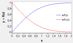
The error function erf(x) and its complement, the complemenatry error function erfc(x), are the lower and upper integrals of the Gaussian function, normalized to unity:

Both functions can be calculated by the NumLib functions speerf and speefc, respectively

function speerf(x: ArbFloat): ArbFloat;   // --> erf(x)
function speefc(x: ArbFloat): ArbFloat;   // --> erfc(x)

Example

A table of some values of the error function and the complementary error function is calculated in the following demo project:

program erf_Table;

uses
  SysUtils, StrUtils, typ, spe;

const
  Wx = 7;
  Wy = 20;
  D = 6;

var
  i: Integer;
  x: ArbFloat;
  fs: TFormatSettings;
begin
  fs := DefaultFormatSettings;
  fs.DecimalSeparator := '.';
  WriteLn('x':Wx, 'erf(x)':Wy+1, 'erfc(x)':Wy+1);
  WriteLn;
  for i:= 0 to 20 do begin
    x := 0.1*i;
    WriteLn(Format('%*.1f %*.*f %*.*f', [
      Wx, x,
      Wy, D, speerf(x),
      Wy, D, speefc(x)
    ], fs));
  end;
end.

Gamma function

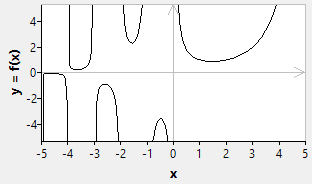
The gamma function is needed by many probability functions. It is defined by the integral

NumLib provides two functions for its calculation:

function spegam(x: ArbFloat): ArbFloat;
function spelga(x: ArbFloat): ArbFloat;

The first one, spegam, calculates the function directly. But since the gamma function grows rapidly for even not-too large arguments this calculation very easily overflows.

The second function, spelga calculates the natural logarithm of the gamma function which is more suitable to combinatorial calculations where multiplying and dividing the large gamma values can be avoided by adding or subtracting their logarithms.

Example

The following demo project prints a table of some values of the gamma function and of its logarithm. Note that spegam(x) overflows above about x = 170 for data type extended.

program Gamma_Table;

uses
  SysUtils, StrUtils, typ, spe;

const
  VALUES: array[0..2] of ArbFloat = (1, 2, 5);
  Wx = 7;
  Wy = 30;
  Wln = 20;

var
  i: Integer;
  x: ArbFloat;
  magnitude: ArbFloat;
begin
  WriteLn('x':Wx, 'Gamma(x)':Wy, 'ln(Gamma(x))':Wln);
  WriteLn;
  magnitude := 1E-3;
  while magnitude <= 1000 do begin
    for i := 0 to High(VALUES) do begin
      x := VALUES[i] * magnitude;
      Write(PadLeft(FloatToStr(x), Wx));
      if x <= 170 then  // Extended overflow above 170
        Write(FormatFloat('0.000', spegam(x)):Wy)
      else
        Write('overflow':Wy);
      WriteLn(spelga(x):Wln:3);
      if abs(x-1000) < 1E-6 then
        break;
    end;
    magnitude := magnitude * 10;
  end;
end.

Incomplete gamma function

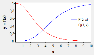
The lower and upper incomplete gamma functions are defined by

In fpc 3.2, these functions were added to NumLib for their calculation

function gammap(s, x: ArbFloat): ArbFloat;
function gammaq(s, x: ArbFloat): ArbFloat;

Example

The following project prints out a table of gammap and gammaq values:

program IncompleteGamma_Table;

uses
  SysUtils, StrUtils, typ, spe;

const
  s = 1.25;

  Wx = 7;
  Wy = 20;
  D = 6;

var
  i: Integer;
  x: ArbFloat;
  fs: TFormatSettings;
begin
  fs := DefaultFormatSettings;
  fs.DecimalSeparator := '.';
  WriteLn('x':Wx, 'GammaP('+FloatToStr(s,fs)+', x)':Wy+1, 'GammaQ('+FloatToStr(s,fs)+', x)':Wy+1);
  WriteLn;
  for i := 0 to 20 do begin
    x := 0.5*i;
    WriteLn(Format('%*.1f %*.*f %*.*f', [
      Wx, x,
      Wy, D, gammap(s, x),
      Wy, D, gammaq(s, x)
    ], fs));
  end;
end.